TycheHowTo:ImportDataIntoGoogleSheets
Let's walk through a process of taking a dataset from an open data site and importing it into a Google Sheets spreadsheet. The purpose of this is to show the end-to-end process and provide a few tips along the eway.
Background
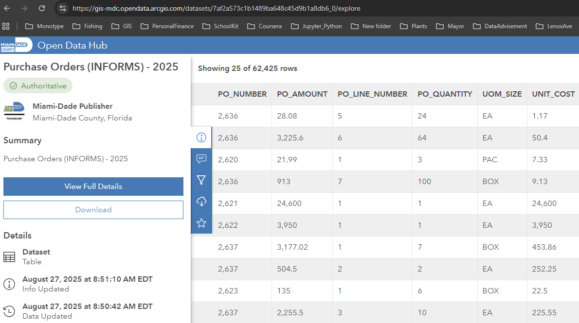
Imagine we are interested in looking at vendor and procurement data for Miami-Dade County. We want to look at the County's purchase orders for goods and services to see when are purchase orders use, what is the typical value of purchase orders, and which vendors are used.
We found a relevant dataset on the Miami-Dade County open data site, shown in the picture above. The dataset lists out purchase orders for 2025. We believe that if we can determine the process for using this data then we can import older data such as the 2024 purchase order data. Looking at the 2025 data we see information such as:
- suppliers - names, addresses
- item descriptions - what was procured, both a short- and long-form description
- purchase order information - identifier,
There are data elements such as "SUPPLIER_PO_TYPE" which seems interesting, however the documentation is not descriptive on the different data values.
Our task is:
- export the data from the Miami-Dade open data system
- import the data into the spreadsheet Google Sheets
- start some basic tests on the data
Exporting the data
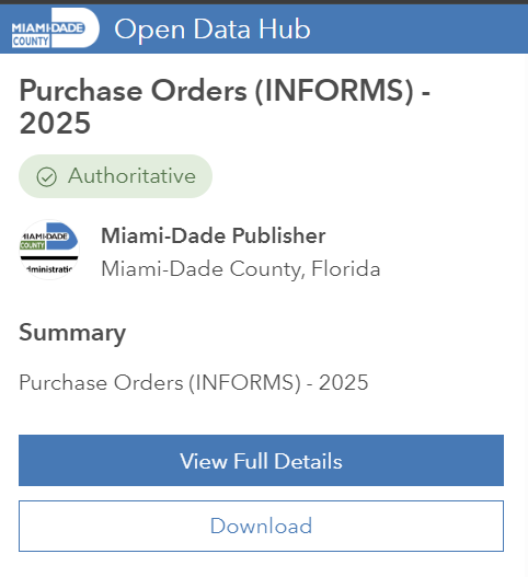
Open data sites typically have either an Export function to download a copy of the data or a recent copy of the data that you can download (or both). The Miami-Dade open data portal has an ability to export date. Click the Download button:
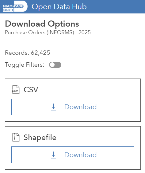
This will provide you with various Download Options. Select CSV to download a comma separated file that can be imported into a spreadsheet:
After you download the file you can open up the file in a text editor. In the example below we have opened the file in Notepad. The highlighted text is the first row with the data or field descriptions; the text below that is the actual data:

The data looks like a good representation of what is found on Miami-Dade's open data site so we are ready to import the data and begin analyzing it.
Importing the data into Google Sheets
For performing work in Google Sheets you will want to create a folder in Google Drive, upload the .csv file to the folder, and create a new Google Sheet. Your folder will look like this:

Open up the Google Sheet, "Miami-Dade County Purchase Orders 2025" or whatever you named it, and choose File > Import within Google Sheets. You will choose your .csv file found in Google Drive:
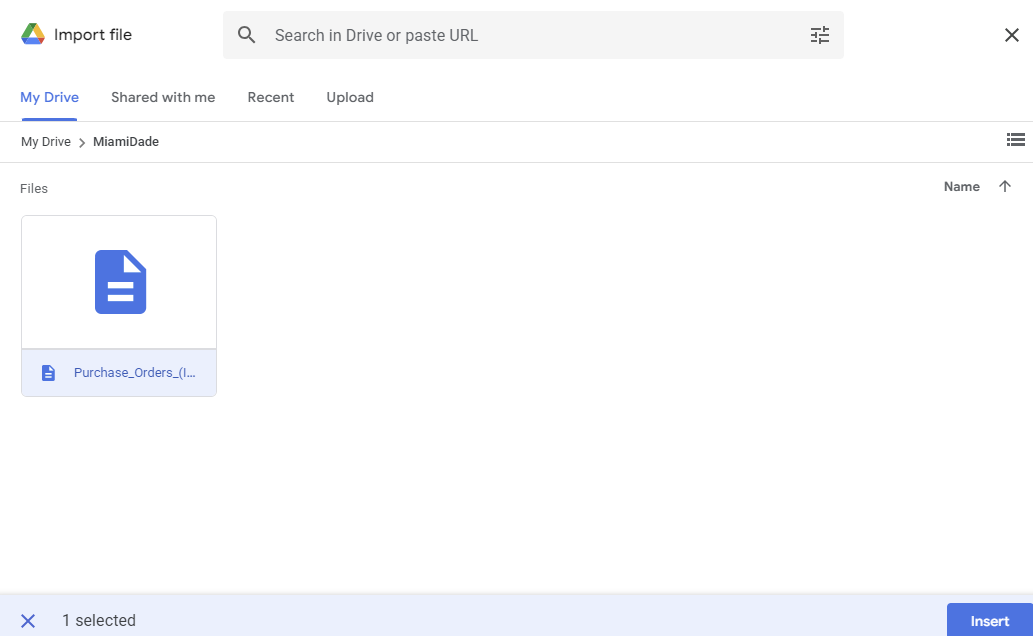
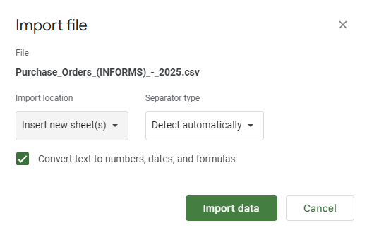
After you click "Insert" you will see some options. We recommend inserting the data into a new sheet and to automatically detect the separator (commas). We also recommend in your first pass choosing to "Convert text to numbers...". This may or may not perform all of the conversions accurately; this is one of the first things to examine.
The .csv data is imported into a new sheet. You can examine the data types or formats for each of the fields. Fields such as PO_NUMBER and PO_AMOUNT are imported correctly as numeric, PO_DATE is a date field, SUPPLIER_NAME and ITEM_DESCRIPTION are character.
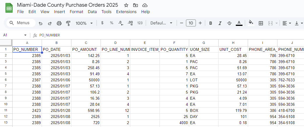
We did find one issue. Row 25 is a suppleir with a New Jersey address; their ZIPCode is 07932 which was is imported in a numeric field as 7932. For the purpose of our analysis we are not going to examine ZIPCode so this is fine for now, however something that needs to be corrected if we do examine ZIPCode.
Lastly, to fully prepare the data for analysis we select all of the data (highlight cell A1 and choose CTRL-A) and choose Data > Create a Filter.
Introductory Data Exploration
We want to test out the data to review both the source data and its importation, and then perform some basic analysis. This will give us confidence for the serious analysis that we want to perform.
As the data has a Filter on it we can test the values of various fields. For example, we can click on the Filter symbol on PO_AMOUNT and sort all purchase orders by their value from the most to least costly.
We have hidden a few fields so that you can see both the PO_AMOUNT and the supplier's information (SUPPLIER_NAME, SUPPLIER_ADDRESS, etc). We can see that there are several large value PO_AMOUNTs associated with the supplier OHLA Building Inc.

One thing to notice is that there are two PO entries with the same PO_NUMBER (5883), the same PO_AMOUNT and the same SUPPLIERT_NAME. We want to understand the potential for double counting. There is another field called PO_LINE_NUMBER; a quick examination suggests that there is a 1:N relationship between a PO_NUMBER and PO_LINE_NUMBER. We can sort the data first by PO_LINE_NUMBER and then by PO_NUMBER to see all entries where PO_NUMBER=5883.
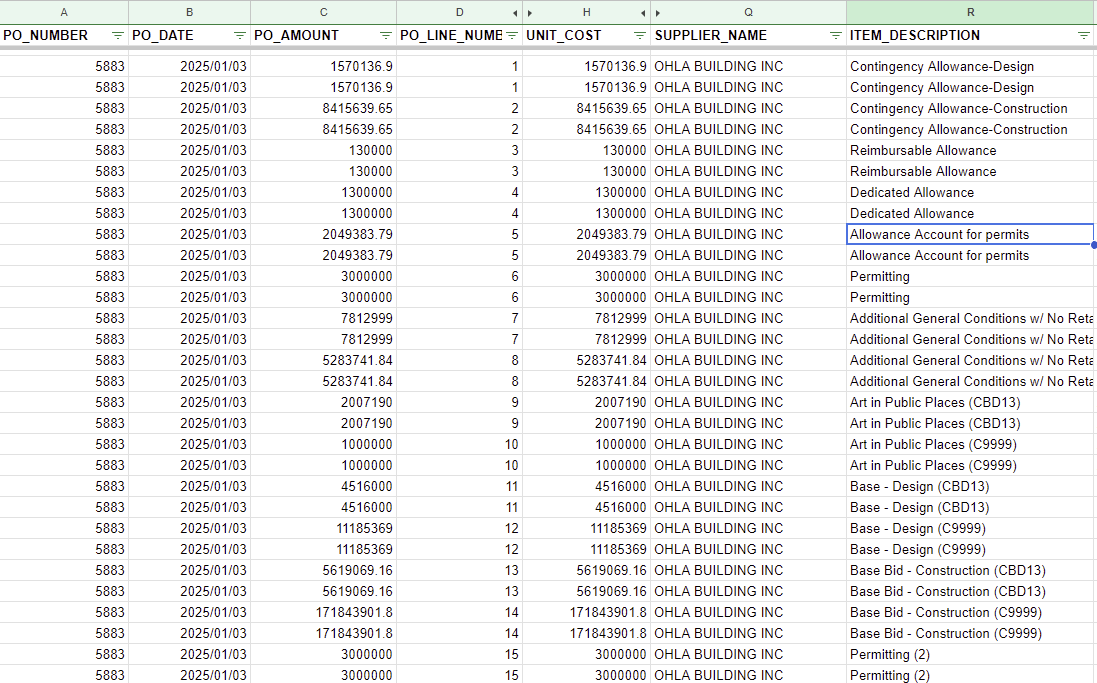
Note that each PO_NUMBER, PO_LINE_NUMBER combination is represented twice in the data. This is something that we'll need to figure out or account for later. However let's not let this get in the way of playing around with the data.
We can perform other tests on the data using different sorting. For example, we can sort PO_DATE to make sure all dates fall within 2025. If we sort PO_DATE - the first PO_DATE = "2025/01/01" the latest date is "2025/03/31"
Testing with pivot tables
Google Sheets Pivot tables are one method to examine data, exercise it, come up with initial findings, and identify underlying issues with the data.
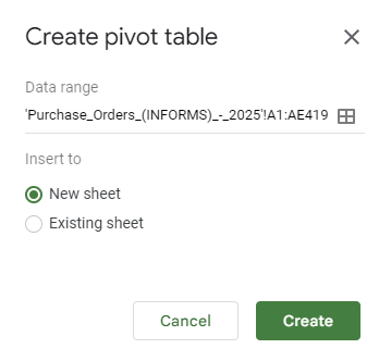
We can select all of our data (highlight cell A1 and choose CTRL-A) and choose Insert > Pivot Table. We can choose to create the pivot table in a new sheet.
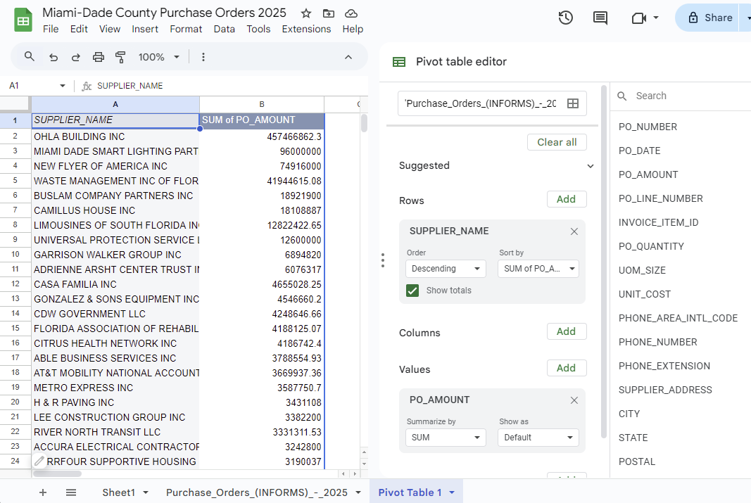
Google Sheets has an interface to configure your pivot table. The first operation we want to look at is the total value of purchase orders by supplier. Note that we will reconcile the potential double entry (noted above) at a later time.
To configure:
- Choose SUPPLIER_NAME as a ROWS
- Choose PO_AMOUNT as a VALUES (ensure that Summarize by is set to SUM)
- Go back to SUPPLIER_NAME and choose Sort by "Sum of PO_AMOUNT", Descending
This will display the pivot table as a list of suppliers with the sum of the value of their purchase orders. OHLA BUILDING INC has the largest value of purchase orders.
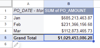
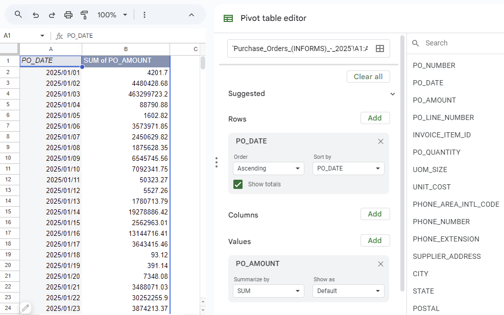
We want to analyze the data in another dimension - value of purchase orders over time. We can create another pivot table that lists out the purchase order month and the value of purchase orders for each month.
To configure the pivot table:
- Choose PO_DATE as a ROWS
- Choose PO_AMOUNT as a VALUES (ensure that Summarize by is set to SUM)
This will display the pivot table as a list of dates with the sum of the value of the purchase orders executed on each date. However this isn't exactly what we want, we would like to group the data by month.
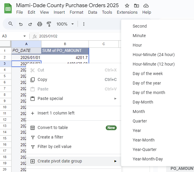
We can highlight any value in the PO_DATE column, right click and choose Create Pivot Date Group > Month.
This will roll up or aggregate the data by month. We can also make a quick change of the formatting of the amounts to be currency, comma serpated. We still have an issue with the double counting of PO values which we will fix at a future point.
